How to Use the Empirical Rule: Full Statistics Guide

Statistics can feel like a maze where numbers wear tiny disguises and wait for you to trip over a formula. Luckily, the empirical rule is one of the friendlier guides in that maze. Also known as the 68-95-99.7 rule, it helps you quickly understand how data behaves when it follows a normal distribution. In plain English: if your data forms a nice bell-shaped curve, the empirical rule tells you where most values are likely to land.

This guide explains how to use the empirical rule step by step, why it matters, when it works, when it does not, and how to solve practical statistics problems without staring at your calculator like it owes you money.

What Is the Empirical Rule?

The empirical rule is a shortcut used in statistics to describe how data is spread around the mean in a normal distribution. It says:

• About 68% of data falls within 1 standard deviation of the mean.
• About 95% of data falls within 2 standard deviations of the mean.
• About 99.7% of data falls within 3 standard deviations of the mean.

That is why the empirical rule is often called the 68-95-99.7 rule. It works best when the data is normally distributed, meaning the graph looks like a smooth, symmetrical bell curve. The mean sits in the middle, and the left and right sides mirror each other like statistical bookends.

Key Terms You Need to Know

Mean

The mean is the average of a data set. Add all the values together, divide by the number of values, and there it isthe mathematical “center of gravity.”

Standard Deviation

Standard deviation measures how spread out the data is. A small standard deviation means values are close to the mean. A large standard deviation means the data is more scattered, like socks after laundry day.

Normal Distribution

A normal distribution is a bell-shaped distribution where most data points cluster near the mean, while fewer values appear farther away. Heights, test scores, measurement errors, and many natural patterns often approximate a normal distribution.

Z-Score

A z-score tells you how many standard deviations a value is from the mean. A z-score of 1 means the value is one standard deviation above the mean. A z-score of -2 means it is two standard deviations below the mean.

How the Empirical Rule Works

Suppose you have a normally distributed data set with a mean of 100 and a standard deviation of 15. Using the empirical rule, you can estimate where most values fall:

• 68% of values fall between 85 and 115.
• 95% of values fall between 70 and 130.
• 99.7% of values fall between 55 and 145.

Here is the math:

• 1 standard deviation: 100 – 15 = 85 and 100 + 15 = 115
• 2 standard deviations: 100 – 30 = 70 and 100 + 30 = 130
• 3 standard deviations: 100 – 45 = 55 and 100 + 45 = 145

With just two numbersthe mean and standard deviationyou can describe a large part of the distribution. That is the power of the empirical rule. It gives you a fast statistical snapshot without requiring a full probability table.

Step-by-Step: How to Use the Empirical Rule

Step 1: Confirm the Data Is Approximately Normal

Before using the empirical rule, check whether the data looks bell-shaped and symmetrical. If the data is heavily skewed, has multiple peaks, or contains extreme outliers, the rule may give misleading results.

A histogram, dot plot, or density curve can help you visually inspect the shape. If the distribution is roughly normal, you can move forward. If it looks like a ski slope, a camel, or a traffic jam, use caution.

Step 2: Identify the Mean

Find the mean of the data set. In many textbook problems, the mean is provided. In real-world analysis, you may need to calculate it yourself.

Formula:

Mean = sum of all values ÷ number of values

Step 3: Identify the Standard Deviation

Next, determine the standard deviation. This tells you how much the data typically varies from the mean. Again, many problems will provide this value. If not, you can calculate it using statistical software, a spreadsheet, or a calculator.

Step 4: Build the Three Main Ranges

Use the mean and standard deviation to create three ranges:

• Mean ± 1 standard deviation
• Mean ± 2 standard deviations
• Mean ± 3 standard deviations

These ranges correspond to 68%, 95%, and 99.7% of the data.

Step 5: Interpret the Results

Once you have the ranges, explain what they mean in context. Statistics is not just about numbers; it is about telling the truth clearly without making the reader run away.

For example, saying “95% of scores fall between 70 and 130” is useful. Saying “the interval bounded by μ ± 2σ contains approximately 0.95 of observations” is also correct, but it sounds like a robot applying for tenure.

Empirical Rule Example: Test Scores

Imagine a statistics exam has scores that are normally distributed. The mean score is 80, and the standard deviation is 5.

• 68% of students scored between 75 and 85.
• 95% of students scored between 70 and 90.
• 99.7% of students scored between 65 and 95.

If a student scored 90, that score is 2 standard deviations above the mean. It is higher than most scores in the class. Not superhero-level rare, but definitely “nice job, maybe explain this chapter to your friends” territory.

Empirical Rule Example: Heights

Suppose adult male heights in a population are approximately normally distributed with a mean of 70 inches and a standard deviation of 3 inches.

• 68% are between 67 and 73 inches tall.
• 95% are between 64 and 76 inches tall.
• 99.7% are between 61 and 79 inches tall.

This example shows why the empirical rule is useful in biology, health research, education, business analytics, manufacturing, and quality control. It gives a quick way to estimate what is typical and what is unusual.

How to Find Percentages Between Specific Values

The empirical rule can also help estimate percentages between parts of the curve. Because a normal distribution is symmetrical, half of the data is below the mean and half is above it.

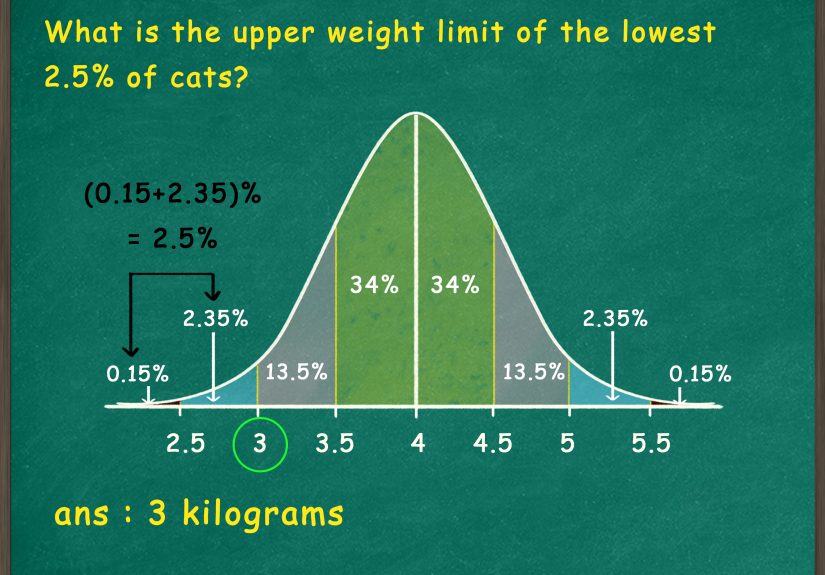
Within 1 standard deviation, 68% of data is centered around the mean. That means 34% lies between the mean and 1 standard deviation above it, and another 34% lies between the mean and 1 standard deviation below it.

Within 2 standard deviations, 95% of data is included. Since 68% is already within 1 standard deviation, the area between 1 and 2 standard deviations on both sides is 27%. Divide that by 2, and each side contains about 13.5%.

Within 3 standard deviations, 99.7% is included. The area between 2 and 3 standard deviations is 4.7% total, or about 2.35% on each side.

Useful Breakdown

• Mean to +1σ: about 34%
• Mean to -1σ: about 34%
• +1σ to +2σ: about 13.5%
• -1σ to -2σ: about 13.5%
• +2σ to +3σ: about 2.35%
• -2σ to -3σ: about 2.35%
• Beyond +3σ: about 0.15%
• Beyond -3σ: about 0.15%

Empirical Rule vs. Chebyshev’s Theorem

The empirical rule applies specifically to normal distributions. Chebyshev’s theorem, on the other hand, works for many distributions, even when they are not normal. However, Chebyshev’s theorem usually gives broader, less precise estimates.

Think of the empirical rule as a sharp kitchen knife: excellent when used correctly, not ideal for every job. Chebyshev’s theorem is more like a sturdy utility tool: less elegant, but more flexible.

When Should You Use the Empirical Rule?

Use the empirical rule when:

• The data is approximately normally distributed.
• You know the mean and standard deviation.
• You need a quick estimate of spread or probability.
• You are analyzing common statistical patterns such as test scores, heights, measurement errors, or quality control data.

It is especially helpful in introductory statistics, AP Statistics, business analytics, psychology, education, and scientific research. It is not a replacement for detailed statistical testing, but it is a very good first look.

When Not to Use the Empirical Rule

Do not rely on the empirical rule when data is strongly skewed, has serious outliers, or does not resemble a bell curve. For example, income data is often right-skewed because a small number of very high incomes pull the average upward. In that case, the empirical rule may create ranges that sound precise but are not very meaningful.

Also be careful with small sample sizes. A tiny data set may look normal by accident, just like three dots can look like a triangle if you want them to badly enough. More data usually gives a better picture of the true distribution.

Common Mistakes Students Make

Mistake 1: Using the Rule on Non-Normal Data

The empirical rule is not universal. It is built for normal distributions. If your data is skewed or irregular, use another method.

Mistake 2: Confusing Standard Deviation with Variance

Standard deviation and variance are related, but they are not the same. The empirical rule uses standard deviation, not variance.

Mistake 3: Forgetting Both Sides of the Mean

The range always extends below and above the mean. “Within 2 standard deviations” means mean minus 2 standard deviations to mean plus 2 standard deviations.

Mistake 4: Treating Estimates as Exact Counts

The empirical rule gives approximate percentages. Real data may not fit the percentages perfectly, even when the distribution is close to normal.

How the Empirical Rule Helps Identify Outliers

Values more than 3 standard deviations from the mean are unusual in a normal distribution. Since about 99.7% of data falls within 3 standard deviations, only about 0.3% falls outside that range.

That does not automatically mean every value beyond 3 standard deviations is wrong. It may be a real rare event. But it does deserve attention. In quality control, finance, science, and data cleaning, these extreme values can signal errors, unusual behavior, or meaningful discoveries.

Real-World Uses of the Empirical Rule

Education

Teachers and testing organizations use normal distributions to understand score patterns. The empirical rule can show whether a student’s score is average, above average, or unusually high or low.

Business

Companies use the empirical rule to monitor performance metrics, customer behavior, delivery times, and product quality. If most delivery times fall within a predictable range, managers can quickly spot delays that are outside the norm.

Manufacturing

In manufacturing, measurements often need to stay within acceptable limits. The empirical rule helps teams understand how much variation is normal and when a process may need adjustment.

Health and Science

Researchers use normal distributions to analyze measurements such as height, blood pressure, lab results, and experimental error. The empirical rule provides a quick way to interpret typical ranges.

Practice Problem

A company tracks daily customer support call times. The call times are normally distributed with a mean of 12 minutes and a standard deviation of 2 minutes.

Question 1: What range contains about 68% of calls?

Use mean ± 1 standard deviation:

12 – 2 = 10
12 + 2 = 14

About 68% of calls last between 10 and 14 minutes.

Question 2: What range contains about 95% of calls?

Use mean ± 2 standard deviations:

12 – 4 = 8
12 + 4 = 16

About 95% of calls last between 8 and 16 minutes.

Question 3: Is a 20-minute call unusual?

Three standard deviations above the mean is:

12 + 6 = 18

A 20-minute call is more than 3 standard deviations above the mean, so it is unusual. It might involve a complex issue, a new employee learning the system, or a customer who decided the support line was also a podcast.

Empirical Rule Formula

The empirical rule is usually written using the mean symbol μ and the standard deviation symbol σ:

• 68%: μ ± 1σ
• 95%: μ ± 2σ
• 99.7%: μ ± 3σ

If you are using sample data, you may see the sample mean written as x̄ and the sample standard deviation written as s. The idea is the same: start at the mean, then move outward by standard deviation units.

Empirical Rule and Z-Scores

The empirical rule connects naturally to z-scores. A z-score tells you how far a value is from the mean in standard deviation units.

Formula:

z = (x – mean) ÷ standard deviation

For example, if the mean is 50, the standard deviation is 10, and a value is 70:

z = (70 – 50) ÷ 10 = 2

That value is 2 standard deviations above the mean. According to the empirical rule, it is higher than most values but still within the range that contains about 95% of the data.

of Practical Experience: Learning to Trust the Bell Curve Without Worshiping It

One of the best ways to understand the empirical rule is to use it with real data, not just textbook examples where every number behaves politely. In real life, data can be messy. It has gaps, surprises, outliers, and occasionally one value that looks like it entered the spreadsheet through a side door. That is why the empirical rule is best treated as a practical guide, not a magical law carved into a calculator.

When students first learn the empirical rule, they often memorize 68, 95, and 99.7 without understanding what those numbers actually do. A better approach is to draw the bell curve and mark the mean in the center. Then add one, two, and three standard deviations on both sides. Suddenly, the rule becomes visual. You can see that most values crowd near the center, while fewer values appear in the tails. This simple picture makes the concept easier to remember than a lonely list of percentages.

In practice, the empirical rule is incredibly useful for quick judgment. Suppose you run a small online store and the average order value is $60 with a standard deviation of $10. If an order comes in at $90, you know it is 3 standard deviations above the mean. That does not automatically mean fraud, celebration, or someone panic-buying socks, but it does tell you the order is unusual compared with the normal pattern. You may want to look at it more closely.

Another helpful experience is comparing the empirical rule with actual data percentages. Take a data set, calculate the mean and standard deviation, then count how many observations fall within one, two, and three standard deviations. If the results are close to 68%, 95%, and 99.7%, your data may be approximately normal. If the results are far away, the distribution may be skewed, flat, heavily tailed, or affected by outliers. This turns the empirical rule into a diagnostic tool, not just a formula.

A common lesson from real analysis is that context matters. For test scores, a value far above the mean may indicate outstanding performance. For machine defects, a value far from the mean may indicate a production problem. For delivery times, an extreme value may signal a traffic delay, staffing issue, or system error. The same statistical distance can mean different things depending on the story behind the data.

The empirical rule is also a confidence builder. Many learners feel statistics is too abstract, but this rule gives them a quick win. Once you know the mean and standard deviation, you can make useful estimates in seconds. That speed is valuable in exams, reports, dashboards, and everyday decision-making.

Still, the smartest analysts stay humble. They check the distribution shape. They watch for outliers. They avoid forcing the empirical rule onto data that clearly does not fit. In other words, they use the bell curve like a flashlight, not a blindfold.

Conclusion

The empirical rule is one of the most useful shortcuts in statistics because it turns the normal distribution into something easy to understand. If you know the mean and standard deviation, you can estimate where 68%, 95%, and 99.7% of values fall. That makes it helpful for interpreting test scores, identifying unusual values, reviewing business performance, analyzing scientific measurements, and understanding variation in everyday data.

The key is knowing when to use it. The empirical rule works best with data that is approximately normal. When the data is skewed, irregular, or full of extreme outliers, use another method or investigate further. Used correctly, the empirical rule is not just a classroom trick. It is a practical tool for making sense of numbers quickly, clearly, and with fewer statistical headaches.